3. Transformation de Green-Riemann
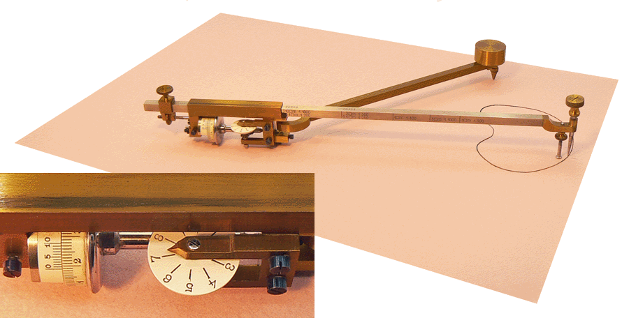
Sur la photographie ci-dessus est représenté un planimètre d'Amsler dont l'utilité est de mesurer l'aire de la courbe fermée
représentée sur la partie droite de la photographie. La partie droite du bras horizontal, dit bras traceur, suit la courbe grâce
à un pointeur vertical.La partie gauche du bras horizontal contient une roulette qui roule sans glisser sur le plan horizontal.
Ce bras horizontal tourne autour d'un point ou passe un bras dit polaire qui se termine par une pointe fixe et lestée par un
cylindre.Nous allons montrer que le nombre de tours de la roulette est proportionnel à l'aire de la courbe fermée.
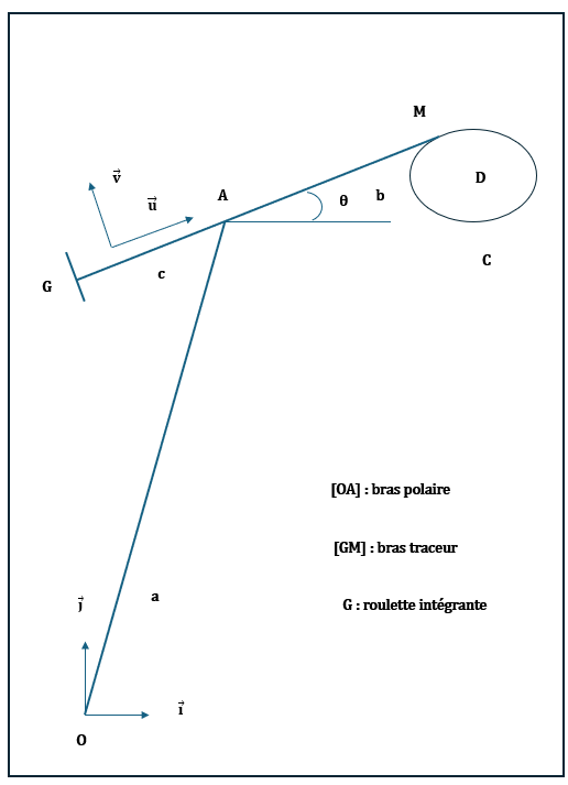
Le dispositif est décrit dans le repère orthonormé \(\mathbf{\left (O,\vec{\imath},\vec{\jmath} \right )}\) et nous aurons besoin de la base mobile \(\mathbf{\left (\vec{u},\vec{v}\right )}\) definie par :
\[\mathbf{\vec{u}=cos(\theta)\, \vec{\imath}+sin(\theta)\, \vec{\jmath}}\]
\[\mathbf{\vec{v}=-sin(\theta)\, \vec{\imath}+cos(\theta)\, \vec{\jmath}}\ .\ \ (2.1)\]
Différentions les vecteurs ci-dessus par rapport à l'angle \(\mathbf{\theta}\) :
\[\mathbf{d\vec{u}=\vec{v}\, d\theta}\]
\[\mathbf{d\vec{v}=-\vec{u}\, d\theta}\ .\ \ (2.2)\]
Ceci étant posé, on peut exprimer le vecteur position de la roulette :
\[\mathbf{\vec{OG}=\vec{OM}+\vec{MG}=\vec{OM}-\left (b+c \right )\, \vec{u}}\ .\ \ (2.3)\]
La projection de \(\mathbf{d\, \vec{OG}}\) suivant \(\mathbf{\vec{v}}\) donne une distance élémentaire parcourue par le centre de la roulette ; Cette
dernière divisée par le rayon de la roulette donne un angle élémentaire de rotation de la roulette autour de son axe.
Intégrons la grandeur, citée ci-dessus sur la courbe fermée :
\[
\begin{align}
\mathbf{\oint_{C}\vec{v}\cdot d\, \vec{OG}}&\mathbf{=\oint_{C}\vec{v}\cdot d\, \left (d\, \vec{OM}-(b+c)\, d\, \vec{u}\right )}\\
&\mathbf{=\oint_{C}\vec{v}\cdot d\, \vec{OM}-(b+c)\, \vec{v}\cdot d\, \vec{u}}\\
&\mathbf{=\oint_{C}\vec{v}\cdot d\, \vec{OM}-(b+c)\, \oint_{C}\vec{v}\cdot d\, \vec{u}}\\
&\mathbf{=\oint_{C}\vec{v}\cdot d\, \vec{OM}-(b+c)\, \underbrace{\oint_{C}\underbrace{\vec{v}\cdot \vec{v}}_{=1}\, d\theta}_{=0}}\\
&\mathbf{=\oint_{C}\vec{v}\cdot d\, \vec{OM}}\ .\ \ (2.4)
\end{align}
\]
Introduisons les décompositions des vecteurs suivants en fonction des vecteurs de base \(\mathbf{\vec{\imath}}\) et \(\mathbf{\vec{\jmath}}\) :
\[
\mathbf{\vec{u}=\dfrac{(x-x_{A})}{b}\, \vec{\imath}+\dfrac{(y-y_{A})}{b}\, \vec{\jmath}}
\]
\[
\mathbf{\vec{v}=\dfrac{-(y-y_{A})}{b}\, \vec{\imath}+\dfrac{(x-x_{A})}{b}\, \vec{\jmath}}
\]
\[
\mathbf{d \, \vec{OM}=dx\, \vec{\imath}+dy\, \vec{\jmath}}\ .\ \ (2.5)
\]
L'expression (2.4) devient avec les relations du (2.5) :
\[
\mathbf{\oint_{C}\vec{v}\cdot d\, \vec{OM}=\dfrac{1}{b}\, \oint_{C}\, -\left ( y-y_{A}\right )\, dx+\left (x-x_{A}\right )\, dy }\ .\ \ (2.6)
\]
La formule de Green-Riemann relie intégration d'une 1-forme \(\mathbf{\omega}\) sur une courbe fermée \(\mathbf{C}\) et intégration de sa
différentielle extérieure(2-forme) \(\mathbf{d\omega}\) sur l'intérieur \(\mathbf{D}\) de la courbe :
\[
\mathbf{\oint_{C}\omega=\iint_{D}d \, \omega}\ .\ \ (2.7)
\]
Appliquons cette relation à l'expression (2.6), il vient :
\[
\mathbf{\oint_{C}\vec{v}\cdot d\, \vec{OM}=\dfrac{1}{b}\, \iint_{D}\left (2-\dfrac{\partial x_{A}}{\partial x}-\dfrac{\partial y_{A}}{\partial y} \right )\, dx \, dy}\ .\ \ (2.8)
\]
Le deuxième membre de l'égalité (2.8) paraît bizzare car il relie les points \(\mathbf{A}\) et \(\mathbf{M}\) mais
cette relation existe à cause des longueurs fixes \(\mathbf{a}\) et \(\mathbf{b}\).
\[\longrightarrow\]
La distance \(\mathbf{OA}\) est fixe de valeur \(\mathbf{a}\) :
\[\mathbf{x_{A}^{2}+y_{A}^{2}=a^{2}}\]
\[\mathbf{x_{A}\, \dfrac{\partial \, x_{A}}{\partial \, x}+y_{A}\, \dfrac{\partial \, y_{A}}{\partial \, x}=0}\ \ \ (1)\]
\[\mathbf{x_{A}\, \dfrac{\partial \, x_{A}}{\partial \, y}+y_{A}\, \dfrac{\partial \, y_{A}}{\partial \, y}=0}\ \ \ (2)\]
\[\longrightarrow\]
La distance \(\mathbf{AM}\) est fixe de valeur \(\mathbf{b}\) :
\[\mathbf{(x-x_{A})^{2}+(y-y_{A})^{2}=b^{2}}\]
\[\mathbf{(x-x_{A})\, \left (1-\dfrac{\partial \, x_{A}}{\partial \, x} \right )+(y-y_{A})\, \left (-\dfrac{\partial \, y_{A}}{\partial \, x} \right )=0}\]
\[\mathbf{(x-x_{A})\, \left (-\dfrac{\partial \, x_{A}}{\partial \, y} \right )+(y-y_{A})\, \left (1-\dfrac{\partial \, y_{A}}{\partial \, y} \right )=0}\]
\[\mathbf{(x-x_{A})\, \dfrac{\partial \, x_{A}}{\partial \, x}+(y-y_{A})\, \dfrac{\partial \, y_{A}}{\partial \, x}=(x-x_{A})}\ \ \ (3)\]
\[\mathbf{(x-x_{A})\, \dfrac{\partial \, x_{A}}{\partial \, y}+(y-y_{A})\, \dfrac{\partial \, y_{A}}{\partial \, y}=(y-y_{A})}\ \ \ (4)\]
\[\longrightarrow\]
Exploitons le système formé des relations (1) et (3) :
\[
\begin{cases}
\mathbf{x_{A}\, \dfrac{\partial \, x_{A}}{\partial \, x}+y_{A}\, \dfrac{\partial \, y_{A}}{\partial \, x}=0}\ \ \ (1)\\
\mathbf{(x-x_{A})\, \dfrac{\partial \, x_{A}}{\partial \, x}+(y-y_{A})\, \dfrac{\partial \, y_{A}}{\partial \, x}=(x-x_{A})}\ \ \ (3)
\end{cases}
\]
On en déduit :
\[
\mathbf{\dfrac{\partial \, x_{A}}{\partial \, x}}=\dfrac{\begin{vmatrix}\mathbf{0}&\mathbf{y_{A}}\\\mathbf{(x-x_{A})}&\mathbf{(y-y_{A})}\end{vmatrix}}{\begin{vmatrix}\mathbf{x_{A}}&\mathbf{y_{A}}\\\mathbf{(x-x_{A})}&\mathbf{(y-y_{A})}\end{vmatrix}}
=\mathbf{\dfrac{x_{A} \, y_{A}-x \, y_{A}}{x_{A} \, y-x \, y_{A}}}\ \ \ (5)
\]
\[
\mathbf{\dfrac{\partial \, y_{A}}{\partial \, x}}=\dfrac{\begin{vmatrix}\mathbf{x_{A}}&\mathbf{0}\\\mathbf{(x-x_{A})}&\mathbf{(x-x_{A})}\end{vmatrix}}{\begin{vmatrix}\mathbf{x_{A}}&\mathbf{y_{A}}\\\mathbf{(x-x_{A})}&\mathbf{(y-y_{A})} \end{vmatrix}}
=\mathbf{\dfrac{x_{A} \, x- x_{A}^{2}}{x_{A} \, y-x \, y_{A}}}
\]
\[\longrightarrow\]
Exploitons le système formé des relations (2) et (4) :
\[
\begin{cases}
\mathbf{x_{A}\, \dfrac{\partial \, x_{A}}{\partial \, y}+y_{A}\, \dfrac{\partial \, y_{A}}{\partial \, y}=0}\ \ \ (2)\\
\mathbf{(x-x_{A})\, \dfrac{\partial \, x_{A}}{\partial \, y}+(y-y_{A})\, \dfrac{\partial \, y_{A}}{\partial \, y}=(y-y_{A})}\ \ \ (4)
\end{cases}
\]
On en déduit :
\[
\mathbf{\dfrac{\partial \, x_{A}}{\partial \, y}}=\dfrac{\begin{vmatrix}\mathbf{0}&\mathbf{y_{A}}\\\mathbf{(y-y_{A})}&\mathbf{(y-y_{A})}\end{vmatrix}}{\begin{vmatrix}\mathbf{x_{A}}&\mathbf{y_{A}}\\\mathbf{(x-x_{A})}&\mathbf{(y-y_{A})}\end{vmatrix}}
=\mathbf{\dfrac{-y_{A}\, y+ y_{A}^{2}}{x_{A} \, y-x \, y_{A}}}
\]
\[
\mathbf{\dfrac{\partial \, y_{A}}{\partial \, y}}=\dfrac{\begin{vmatrix}\mathbf{x_{A}}&\mathbf{0}\\\mathbf{(x-x_{A})}&\mathbf{(y-y_{A})}\end{vmatrix}}{\begin{vmatrix}\mathbf{x_{A}}&\mathbf{y_{A}}\\\mathbf{(x-x_{A})}&\mathbf{(y-y_{A})} \end{vmatrix}}
=\mathbf{\dfrac{x_{A} \, y- x_{A}\, y_{A}}{x_{A} \, y-x \, y_{A}}}\ \ \ (6)
\]
On peut maintanant calculer :
\[
\mathbf{2-\dfrac{\partial \, x_{A}}{\partial \, x}-\dfrac{\partial \, y_{A}}{\partial \, y}=2-\dfrac{x_{A} \, y _{A} -x \, y_{A}}{x_{A} \, y-x \, y_{A}}-\dfrac{x_{A} \, y-x_{A} \, y_{A}}{x_{A} \, y-x \, y_{A}}=1}
\]
La relation (2.8) se simplifie en :
\[
\begin{align}
\mathbf{\oint_{C}\vec{v}\cdot d\, \vec{OM}}&\mathbf{=\dfrac{1}{b} \, \iint_{D}(2-1) \, dx \, dy}\\
&\mathbf{=\dfrac{1}{b} \, Aire(D)}\ .\ \ (2.9)
\end{align}
\]
Ainsi l'angle balayé par la roulette est proportionnel à l'aire de la courbe fermée parcourue par la pointe.